CORRELATION NOTES PDF: Correlation, Correlation and Causation, Types of Correlation, Significance of Correlation, Methods of Correlation etc.
CORRELATION
Correlation is a statistical technique which shows the degree and direction of relationship between the two variables. It ranges between -1 to +1.
According to AM Tuttle
“Correlation is the analysis of co-variation between two or more variables.”
According to Croxton and Cowden
“When the relationship is of a quantitative nature, the appropriate statistical tool for discovering and measuring the relationship and expressing it in a brief formula is known as correlation.”
Thus, whenever two variables are so related that a change in the value of one is accompanied by a change in the value of the other, in such a way that
(a) an increase or decrease is one variable is accompanied by an increase or decrease in the other or
(b) a fall in one variable is accompanied by a fall or rise in the other, then the variables are said to be correlated.
SIGNIFICANCE OF CORRELATION
The significance or utility of correlation is clear from the following points:
HELPS IN MEASURING THE EXTENT OF RELATIONSHIP: The correlation coefficient helps us in measuring the extent of relationship between two or more than two variables. The degree and extent of the relationship between two variables is, of course, one of the most important problems in statistics.
HELPS IN PREDICTIONS: It is through correlation that we can predict about the future. For instance, if there are good monsoons, we can expect better food supply and hence can expect fall in price of food grains and other products. The predictions made on the basis of correlation analysis are considered to be nearer to reality and hence reliable. In the words of Tippett. “The effect of correlation is to reduce the range of uncertainty of our prediction.”
HELPS IN STUDYING ECONOMIC BEHAVIOR: Correlation contributes to economic behaviour. It helps us in knowing the important variables on which others depend.
HELPS IN FURTHER STATISTICAL TREATMENT: The technique of ratio of variation and regression analysis depends totally on the findings of coefficient of correlation.
HELPFUL IN FIELD OF COMMERCE AND INDUSTRY: In the field of commerce and industry, the technique of correlation coefficient helps to make estimates like sales, price or costs.
The predictions made on the basis of correlation analysis are considered to be nearer to reality and hence reliable. In the words of Tippett. “The effect of correlation is to reduce the range of uncertainty of our prediction.”
Thus, the technique of correlation coefficient is the most useful tool in statistical analysis in every discipline. In the words of W.A. Neiswanger, “Correlation analysis contributes to the understanding of economic behaviour, aids in locating the critically important variables on which other depend, may reveal to the economists the connections by which disturbances spread and suggest to him the paths through which stabilising forces may become active.”
TYPES OF CORRELATION
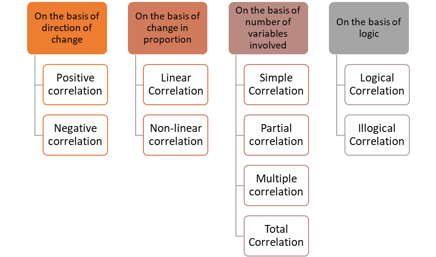
ON THE BASIS OF DIRECTION
Positive or direct correlation:
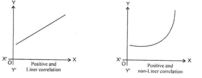
If the two variables move in the same direction i.e. the other variable also falls, the correlation is said to be positive. For example, price and supply are positively related.
It means if price goes up, the supply goes up and vice versa.
| Price | Supply |
| 50 | 100 |
| 60 | 120 |
| 70 | 140 |
| 80 | 160 |
| 90 | 180 |
The above illustration shows that as price increases the supply also increases and vice-versa.
Diagrammatically, it can be shown as follows:
Negative or Inverse Correlation:
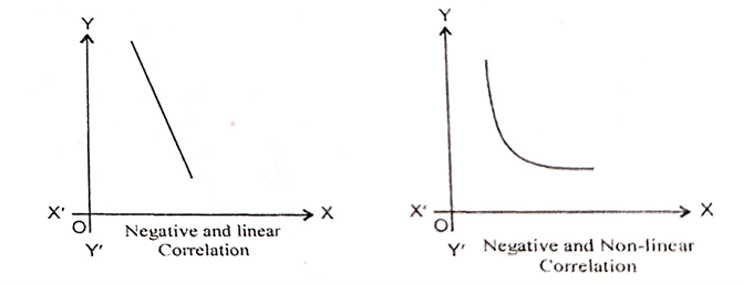
If two variables move in opposite direction i.e. with the increase in one variable, the other variable falls or with the fall in one variable, the other variable rises, the correlation is said to be negative or inverse. For example, the law of demand shows inverse relation between price and demand.
| Price | Demand |
| 50 | 180 |
| 60 | 160 |
| 70 | 140 |
| 80 | 120 |
| 90 | 100 |
The above illustration shows that as price increases the demand decreases and vice-versa.
ON THE BASIS OF NUMBER OF VARIABLES
Simple Correlation
When there are only two variables and the relationship is studied between those two variables, it is a case of simple correlation Relationships between height and weight, price and demand or income and consumption étc. are examples of simple correlation
Multiple Correlation
When there are more than two variables and we study the relationship between one variable and all the other variables taken together then it is a case of multiple correlation. Suppose there are three variables 1, 2, 3 we can study the multiple correlation between A and B & C taken together or between B and A & C together etc. It can be denoted as r 1.23 or r2.13 or r3.12.
Partial Correlation
When there are more than two variables and the relationship between any two of the variables is studied assuming other variables as constant it is a case of partial correlation. This, in fact, is an extension of multiple correlation. Suppose we study the relationship between rainfall and crop, without taking into consideration the effects of other inputs like fertilizers, seeds and pesticides etc., this technique will be known as partial correlation. Symbolically if x, y, z are the three variables then partial correlation between x and y excluding z will be given by rxy.z, rxz.y or ryz.x
Total Correlation
When the correlation between the variables under study taken together at a time, is worked out, it is called total correlation.
The main point worth consideration is that this line will indicate positive relation if ‘a’ is positive and in case ‘a’ is negative the correlation will also be negative. In such type of correlation, the value of the coefficient of correlation is always + 1 or 1 depending on the sign of ‘a’ in the equation of y = ax + b. Correlation will be + 1 if ‘a’ is +ve and -1 if ‘a’ is -ve.
ON THE BASIS OF CHANGE IN PROPORTION
Linear Correlation
Linear correlation is said to exist if the amount of change in one variable tends to bear a constant ratio to the amount of change in the other variable.
| X | Y |
| 5 | 10 |
| 10 | 20 |
| 15 | 30 |
| 20 | 40 |
| 25 | 50 |
Thus, it is clear from the above that the ratio of change between the two variables is the same. If such variables are plotted on a graph paper all the plotted points would fall on a straight line.
Diagrammatically, it can be shown as follows:
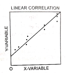
This type of relation does not exist in economics and other social sciences. This type of relation can exist in only physical sciences. However, it has great theoretical importance in economics and other social sciences.
Non-Linear Correlation
Non-linear correlation is said to be curvi-linear correlation when the proportion of change in two variables is not proportional. For example, if we double the amount of rainfall, the proportion of rice and wheat etc. would not necessarily be proportional.
| X | Y |
| 5 | 10 |
| 10 | 13 |
| 15 | 17 |
| 20 | 18 |
| 25 | 21 |
| 30 | 29 |
Thus, from the above example it is clear that the ratio of change between two variables is not the same. Now, if we plot all these variables on a graph, they would not fall on a straight line.
Diagrammatically, it can be shown as follows:
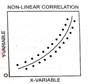
Such types of correlations are found very commonly in the fields of economics and the other social sciences. As such these are very important in the study of social sciences.
ON THE BASIS OF LOGIC
Logical Correlation
When the correlation between two variables is not only mathematically defined but also logically sound too, it is called logical correlation. For example, correlation between income and consumption, price and demand, age and playing habits etc. are logical correlations. These correlations are determined by both ways mathematically as well as logically. In other words, it can be said that the correlations in the above cases whether negative or positive can be confirmed by logic or by applying the requisite statistical tools of correlation. There exists functional relationship between the variables.
Illogical Correlation
In certain cases we come across such cases of relationship of variables which are though well defined and established by statistical method of correlation coefficient, yet when tested on the logical point of view they fail to justify their relationship with each other. For example relationship between rainfall and the number of babies born. production of cycles and the death rate. etc. These variables are not connected with each other in any way. But their correlations can be established by applying the statistical methods of correlation. Such type of correlation is known as Non-Sense Correlation or Spurious correlation.
DEGREES OF CORRELATION
According to Karl Pearson, the coefficient of correlation lies between two limits i.e. +1 and -1. It implies that there is perfect positive relationship between two variables, the value of correlation would be positive one. On the contrary, if there is perfect negative relationship between two variables the value of the correlation will be negative one. It means r lies between +1 and -1. Within these limits the value of correlation can be interpreted as:
| r=+1 | Perfect Positive Correlation |
| r>+0.75 but < +1 | High degree of positive correlation |
| r>+0.5 but < +0.75 | Moderate degree of positive correlation |
| r> +0 but <+0.5 | Low degree of positive correlation |
| r=0 | No correlation at all |
| r>-0.75 but < -1 | High degree of negative correlation |
| r>-0.5 but < -0.75 | Moderate degree of negative correlation |
| r> -0 but <-0.5 | Low degree of negative correlation |
| r=-1 | Perfect negative correlation |
PRESENCE OF CAUSATION RESULTS IN CORRELATION – CORRELATION AND CAUSATION
The construction of a scatter diagram and the calculation of the coefficient of Correlation merely establish the fact that the two variables are associated in their magnitude but it does not manifest functional relationship. The presence of correlation between two variables or series does not mean cause and effect relationship. But the presence of causation always results in Correlation. Therefore, the coefficient of correlation must be taken as a measure of co-variation. Whether the correlation found reflects an important casual relation is a matter of careful interpretation in the light of our general knowledge about the data.
Any one of the following factors may cause correlation.
1. Cause and effect relationship: For such variables which are mutually influencing each other, it is difficult to establish cause and effect relationship. For example, when the price of the commodity gets up demand for that commodity goes down. Here price is the cause and demand is the effect. This other way is also possible. In many cases, the increased demand for a commodity raises the price. Now demand is the case and price are effect.
The variable which is supported to be the cause for the change in the second variable if called independent variable and is plotted upon horizontal axis. The second related variable is called dependent variable and is plotted along vertical axis for such variables, the coefficient of correlation does not the any light whether. Variable X causes variable Y or variable Y causes variable X
2. Common factor: Two variables may be correlated not because of direct relationship but because each variable is related to the same third variable. Each variable may be affected either in the same way or in the different way by the common third variable. For Example, there is a negative correlation between the demand for X commodity and Supply of Y commodity because of the fact that both are related to price. Similarly high degree of correlation exists between the per acre yield of rice and wheat due to the fact that both variables are related to the common variable irrigation.
3. Correlation between two variables may be due to sampling fluctuations: In same cases there may be no relationship between variables in the population from which the sample is drawn. But samples values of both variables may show some degree of relationship due to sampling fluctuation. Thus it might be found that in a group of male students, there may exists positive correlation between the amount of money in their pockets and long hair styles. Yet it is difficult to say why it is so and the chances are that the second sample may produce totally different results.
4. Interdependent Relationship: In many situation, correlation between two variables may be the result of Interdependent relationship. This is situations where two variables interact i.e. change in one variable causing changes in the second variable which is than cause change in the first variable and so on For example, a high price of a commodity stimulates its production; but increased production many increase or decrease the cost of production of a commodity and through the change in cost the price of a commodity will be affected.
CORRELATION COEFFICIENT
The coefficient of correlation may be defined as the measurement of the degree of relationship between two variables. It indicates the directions as well as closeness of relationship between two variables. It is denoted by the symbol ‘r’ and always varies between +1 and -1.
METHODS OF CALCULATING CORRELATION COEFFICIENT
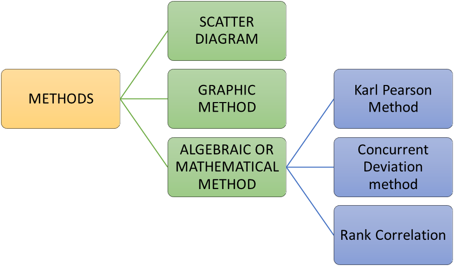
SCATTER DIAGRAM METHOD
Diagrammatic or scatter diagram is the simplest way of showing bivariate distribution and evaluating the correlation on the basis of the corresponding values of any two variables. Suppose we are given two variables A and B. The value of A are represented by the X axis and value of B on Y axis. Through normal scale on which equal division shows equal values. For each pair (A1, B1), (A2, B2), (A3,B3,) ………. AnBn points may be plotted as dots (•) on X and Y axis in the XY plan. The diagram of dots so takers is called Scatter diagram. It gives us a estimated or rough idea about the relationship of two variables.
Take dependent variable along the Y axis and an independent variable along the X axis.
INTERPRETATION OF SCATTER DIAGRAM
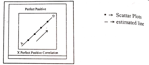
In case, the plotted points from a straight line AB rising from the lower left hand corner to the upper right hand corner as depicted, there exists a perfect positive correlation between two variables. For such variables, the coefficient of correlation is +1 (r = +1)
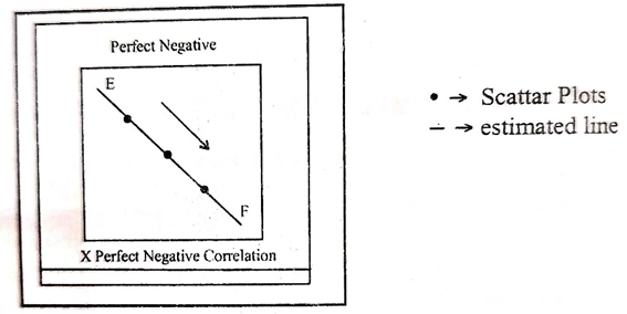
If all the plotted dots lies on a straight line EF falling from upper left hand corner to lower right hand corner as shown in figure, there is perfect negative correlation between the two variable. In this ca the coefficient of correlation takes the values of -1 (r-1).
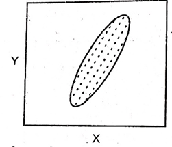
If the plotted points in the plane from a band and they show a rising trend from the lower left hand corner to upper right hand corner as shown in figure, the top variables are positively correlated. The degree of relationship depends upon the structure of band i.e. narrower the band higher degree of relationship between the two variables and looser the band, lower the degree of relationship between the two variables.
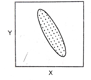
If the plotted dots in the plane from a band and they show a falling trend from upper left hand corner to the lower right hand corner as shown in figure there is negative correlation between the two variable. The degree of relationship depend upon the structure of band i.e. narrower the band higher the degree of negative correlation and looser the band, lower the degree of negative correlation.
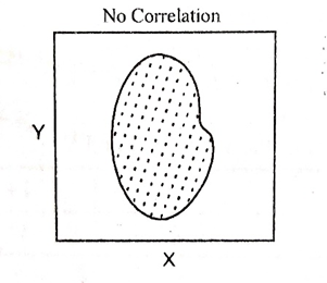
If the plotted points in the plane are spread all over the diagrams shown in the figure. The variables are not correlated. Such variables are independent.
MERITS OF SCATTER DIAGRAM METHOD:
(1) Simple Method: The scatter diagram is the simplest method of studying correlation between two variables.
(2) Easy to Understand: It is much easier to understand compared to complex mathematical formulae involved in the calculation of correlation coefficient.
(3) No effect of extreme values: The scatter diagram is not affected by items of extreme size.
LIMITATIONS OF SCATTER DIAGRAM METHOD:
- No Numerical Expression of relationship: The scatter diagram indicates only the direction of the correlation between two variables but it is silent about the magnitude of relationship. Thus it falls to provide a numerical measure of correlation.
- This method is not suitable when the number of observations are sufficiently large.
SUITABILITY OF SCATTER DIAGRAM METHOD:
The scatter diagram for studying relationship between two variables is mainly used when we are interested only in getting rough idea about the nature of relationship between two variables. In addition to this, it is also used when the results are needed immediately about the nature of relationship.
GRAPHIC METHOD
According to this method the graph of two series are drawn on the same graph paper according to some suitable scale i.e.
1. Natural Scale
2. Ratio Scale
3. Semi-logarithmic Scale depending on the size of the data.
If the two graphs run parallel to each other left to right whether in the upward direction or in the downward direction, the correlation is said to be perfect positive. If the graphs are in the opposite direction the correlation will be negative.
If minimum value of variables are much higher than zero, a false base may be drawn to avoid non required empty space.
The method is the most undependable and cannot be put any further use. We can roughly observe the relationship only from the movement of the two graph. If the two graphs are parallel the correlation is positive. If the movements in the graph of two series shows an opposite trend that is if of one goes up while the other falls the correlation will be said to be negative.
Although the two extreme cases of correlation perfect positive correlation and perfect negative correlation and perfect negative correlation are quite visible to determine by this graph but in other moderate cases we can judge the correlation precisely. In such cases the points of maxima and minima will be different if we try to establish the fact with regards to the turning points on the two curves.
Correlation between the two curves can be expressed graphically as under:

INTERPRETATION
1. If both lines of variable drawn on the graph moves in the same direction, i.e., either upward or downward, it is said to be positive correlation.
2. If both the lines drawn on the graph moves in the opposite direction i.e., one moves upward and other moves downward, it shows a negative correlation.
3. If both the lines drawn on the graph shows erratic movement it shows no correlation (or low correlation)
MERIT OF GRAPHIC METHOD:
The nature and extent of the correlation from a graph can be determined.
DEMERIT OF GRAPHIC METHOD:
The exact degree of correlation cannot be determined by this method.
SUITABILITY OF THIS METHOD:
This method is used where the data is given over a period of time and where the exact degree of correlation is not needed.
ALGEBRAIC OR MATHEMATICAL METHOD
KARL PEARSON’S METHOD
Karl Pearson, a reputed statistician, in 1890, has constructed a well set formula based on mathematical treatment for determining the coefficient of correlation. The formula is named after his name as Karl Pearson’s formula and is popularly known as ‘Karl Pearson’s coefficient of correlation. It is also named as, ‘Product moment coefficient.
CHARACTERISTICS OF KARL PEARSON’S COEFFICIENT OF CORRELATION
Following are the main characteristics of Karl Pearson’s Coefficient of Correlation.
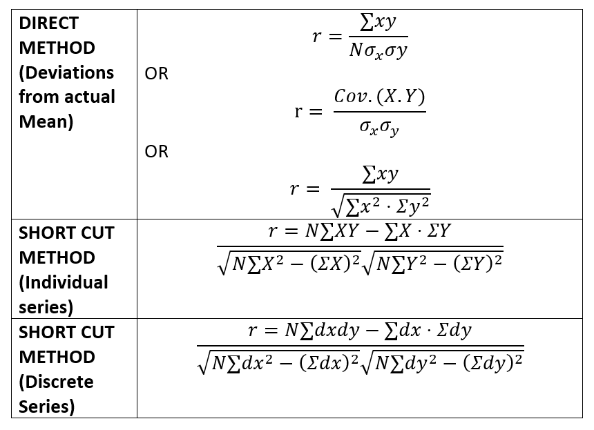
1. Based on Arithmetic Mean and the Standard Deviation: The formula is based upon arithmetic mean and standard deviation. The products of the corresponding values of the two series i.e. co-variance is divided by the product of standard deviations of the two series to determine the formula.
2. Determines the direction of relationship: Karl Pearson’s method establishes the direction of relationship of variables viz., Positive or Negative.
3. Establishes the Size of relationship: Karl Pearson’s method also shows the size of relationship between variables of the two series. It ranges between +1 and -1. +1 means perfect positive correlation and -1 means perfect negative relationship. In case the value is ‘0’ then it means no relationship between the variables.
4. Ideal Measure: Karl Pearson’s method is considered to be an ideal method of calculation of correlation coefficient. It is because of the covariance which is most reliable as a standard statistical tool.
PROPERTIES OF KARL PEARSON’S COEFFICIENT
The following are the main properties of Karl Pearson’s coefficient of correlation:
1. In case correlation is present, then coefficient of correlation would lie between +1 and -1. If correlation in absent, then it is denoted by zero.
2. Coefficient of correlation is based on a suitable measure of variation as it takes into account all items of the variable.
3. Coefficient of correlation measures both-the direction as well as degree of change.
4. If there is accidental correlation, in that case the coefficient of correlation might lead to fallacious conclusions. It is known as nori-sense or spurious correlation.
5. The coefficient of correlation does not prove causation but it is simply a measure of co-variation. It is because variations in X and Y series may be due to,
(i) some common cause,
(ii) some mutual dependence,
(ii) some change, and
(iv) some causation of the subject to be relative.
6. It is independent of changes of scale and origin of the variables X and Y.
7. Coefficient of correlation is a geometric mean of two regression coefficients. Symbolically

8. Coefficient of correlation is independent of the unit of measurement.
9. Coefficient of correlation works both ways
i.e. rxy=ryx
10. If the value of x and y are linearly related with each other i.e, if we have the relation between x and y as y=ax + b, the correlation coefficient between x and y will be +1 and if the relation between x and y is as y=-ax + b, then r will be -1, ‘a’ being negative constant.
ASSUMPTIONS OF COEFFICIENT OF CORRELATION
Coefficient of correlation of Karl Pearson is based on the following assumptions:
1. The relationship is linear: There is a linear relationship between the two variables. That means if the two variables are plotted, we get a straight line
2. Normal Distribution. A large number of independent causes are operating in both the variables correlated so as to produce a normal distribution.
3. Related in a casual fashion: There is a cause and effect relationship between the forces affecting the distribution of the items in the two series, If these forces are independent, there cannot be any correlation.
CALCULATION OF KARL PEARSON COFFICIENT OF CORRELATION
MERITS OF KARL PEARSON COEFFICIENT OF CORRELATION
Karl Pearson’s coefficient of correlation has the following merits.
(1) Counts all Values: It takes into account all values of the given data of x and y. Therefore, it is based on all observations of the series.
(2) More Practical and Popular: Karl Pearson’s ‘r’ is considered to be more practical method as compared to other mathematical methods used for ‘r’. It is also very popular and as such, commonly used method.
(3) Numerical Measurement of ‘r’: It provides numerical measurement of coefficient of correlation.
(4) Measures Degree and Direction: This method measures both degree and direction the correlation between the variables at a time.
(5) Facilitates Comparison: Karl Pearson’s coefficient of correlation is a pure number -independent of units. Therefore, the comparison between the series can be done easily.
(6) Algebraic treatment Possible: Karl Pearson’s coefficient of correlation techniques can easily be applied for higher algebraic treatment.
DEMERITS OF KARL PEARSON COEFFICIENT OF CORRELATION
The use of coefficient of correlation has certain limitations which are as under:
- Linear Relationship: Coefficient of correlation assumes linear relationship between the variables regardless of the fact whether that assumption is correct or not.
- More time Consuming: Compared with some other methods, this method is more time consuming.
- Affected by extreme items: Another drawback of coefficient of correlation is that it affected by the extreme items.
- Difficult to interpret: It is not easy to interpret the significance of correlation coefficient. It is generally misinterpreted.
RANK CORRELATION
This method was developed by the British Psychologist Prof. Charles Edward Spearman in 1904. Rank correlation coefficient is used for measuring the relationship between two qualitative variables such as honesty, beauty, taste etc., which cannot be measured quantitatively. This method is used when ordinal (rank) data are available. This method is known as ‘Spearman’s coefficient of correlation or popularly known as ‘Rank Correlation. The data are quite irregular in case of qualitative aspects.
Rank Correlation is denoted by rs or p (rho).
Formula to calculate Rank Correlation is as follows:

CHARACTERISTICS OF RANK CORRELATION COEFFICIENT
The following are the main features or properties of rank correlation coefficient:
1. Like Karl Pearson’s coefficient of correlation, Spearman’s rank correlation coefficient also lies between – 1 to +1.
2. Sum of difference of ranks between two variables is zero i.e. Sum of D=0.
3. It is not based on the assumption of normal distributions of population.
4. When Sum of D2=0, p = 1. It means each D= 0 and both series have similar ranks.
MERITS OF RANK CORRELATION COEFFICIENT
- It is easy to understand and simple to calculate.
- Where measurements are given in the quantitative form, there too this method can be used by assigning ranks to different values.
- In the study of relationship of series having qualitative characteristics such as beauty, honesty, tastes, promotions etc., Rank correlation method is the only substitute.
DEMERITS OF RANK CORRELATION COEFFICIENT
- It has no further application in any statistical operation.
- We cannot determine combined coefficient of correlation based upon the values of a few samples.
- Spearman’s coefficient of correlation can’t be applied in case of grouped frequency distribution.
- It is not an approximate measure of correlation because it is not based on the actual values in the data.
CONCURRENT DEVIATION METHOD
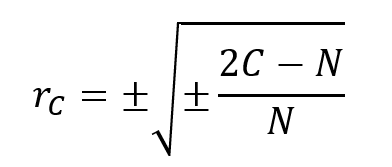
Amongst all the methods of calculating coefficient of correlation, concurrent deviation method is the simplest method. By this method we simply observe the direction of each value in each series with reference to the preceding value. If the next value rises we put + sign before it and if it decreases we put sign before it. If the value remains stationary i.e. there is no change at any stage we put ‘0’ before Here N is not the number of pairs of X and Y values.
It is always one less than the number of pairs because we have to leave the first pair because of the inability to establish its trend. After recording the +ve and-ve movements we multiply the two. The resultant series will give +ve sign if there is similar movement in both series ie either both +ve or both-ve and Number of times gives-ve sign if there is reverse movement in the two series one +ve and other-ves. We call the concurrent deviations in the two series. These concurrent deviations are represented by ‘c’.
The formula for calculating coefficient of correlation by this method is:
MERITS OF CONCURRENT DEVIATION METHOD
- It is the simplest and easily understandable method of measuring correlation.
- If no further analysis is to be made this method is the most suitable to establish the correlation between two variables.
- It gives correct indication as to the direction and degree of the correlation.
- It does not depend upon the normality assumption.
DEMERITS OF CONCURRENT DEVIATION METHOD
- It is a rough measure of correlation and as such cannot be put to any further analysis.
- This method does not give any weightage to the changes or the magnitude of the deviations of the items from the preceding values. All changes big or small are treated at per which has no logic at all.
- If we calculate coefficient of correlation for two or more samples from the same universe, this formula fails to find out the combined coefficient for all the samples taken together.
- This method is not based on all values in series.
| Also Study: | Also Study: | Also Study: | Also Study: | Also Study: |
| Measures of central tendency | Arithmetic Mean | Median | Mode | Statistics |
| Functions of statistics | Scope of statistics | Limitations of Statistics | Distrust of statistics | INTRODUCTION TO STATISTICS |
| MEASURES OF CENTRAL TENDENCY BCOM NOTES |