LINEAR PROGRAMMING TERMS AND DEFINITIONS
LINEAR PROGRAMMING
Linear programming deals with the optimization (maximization or minimization) of a linear function, called objective function, involving number of variables, subject to the set of variables, subject to the set of linear equalities and for inequalities called constraints and variables should be non-negative.
ACCORDING TO SAMUELSON AND SLOW
“ The analysis of problems in which a linear function of variables is to be maximised or minimised when these variables are subjected to number of constraints in the form of linear inequalities.”
ACCORDING TO WILLIAM M. FOX
“Linear programming is a planning technique that permits some objective function to be minimized or maximized within the framework of given situational restrictions.”
In linear programming, ‘Linear’ means that all the relation used in the problems are linear whereas ‘programming’ stands for the process of finding a plan of action.
UNBOUNDED SOLUTION IN SIMPLEX METHOD
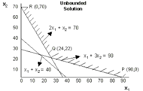
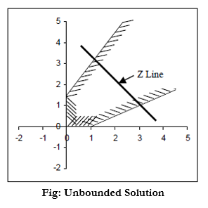
An unbounded solution in the simplex method of linear programming refers to a situation where the objective function can be improved without limit, that is, there is no finite optimal solution to the problem.
In the simplex method, we start with an initial feasible solution and iteratively improve it by pivoting among the basic variables until we reach an optimal solution. However, if the objective function can be improved indefinitely, the problem is said to be unbounded.
There are several reasons why a linear programming problem might have an unbounded solution. One possible reason is that the feasible region is unbounded, meaning that there is no upper bound on one or more of the decision variables. Alternatively, it could be due to constraints that are redundant or inconsistent, which allows the feasible region to extend infinitely.
To determine whether a linear programming problem has an unbounded solution, we can examine the final simplex tableau after we have obtained the optimal solution. If there is at least one negative coefficient in the objective row, this indicates that the objective function can be improved by increasing the corresponding non-basic variable. If all non-basic variables have nonnegative coefficients, then the problem has an optimal solution. However, if there is at least one non-basic variable with a negative coefficient, the problem is unbounded.
FEASIBLE ZONE IN LINEAR PROGRAMMING
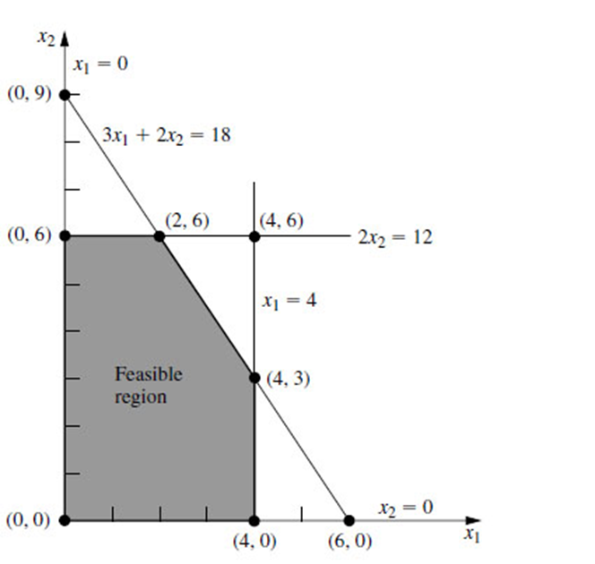
In linear programming, the feasible region (or feasible set or feasible solution space) refers to the set of all possible solutions that satisfy the constraints of a given linear programming problem. The feasible region is defined by the intersection of the constraints, and it is typically represented graphically as a polygon (or polyhedron in higher dimensions) in the space of decision variables.
More specifically, the feasible region is the set of all points (x1, x2, …, xn) that satisfy the system of linear inequalities:
a11x1 + a12x2 + … + a1nxn ≤ b1 a21x1 + a22x2 + … + a2nxn ≤ b2 … am1x1 + am2x2 + … + amnxn ≤ bm
where aij and bi are known coefficients and xi are the decision variables. The feasible region is a subset of the n-dimensional space of decision variables that satisfies all of the above inequalities simultaneously.
The feasible region is important in linear programming because the optimal solution (i.e., the solution that maximizes or minimizes the objective function) must lie within the feasible region. Therefore, the feasible region provides a way to identify the range of feasible solutions and to search for the optimal solution within that range.
The feasible region can be found graphically by plotting the constraints and identifying the region of the plane (or space) that satisfies all the constraints simultaneously. In two dimensions, for example, the feasible region is a polygon formed by the intersection of the constraint lines. In three dimensions, the feasible region is a polyhedron formed by the intersection of the constraint planes, and so on.
The feasible region can also be found algebraically by solving the system of inequalities using techniques such as Gaussian elimination, linear programming algorithms, or other optimization methods.
In summary, the feasible region in linear programming is the set of all possible solutions that satisfy the constraints of a given problem, and it is important for identifying the range of feasible solutions and searching for the optimal solution within that range.
NON-NEGATIVITY CONSTRAINTS IN LINEAR PROGRAMMING
Non-negativity constraint is a restriction in a linear programming problem stating that negatives values for physical quantities cannot exist in a solution.
The linear inequalities x≥0 and y≥0. These are included because ‘n’ and ‘y’ are usually the number of items produced and it is not possible to produce negative number of products or the smallest number of products or the smallest number of items could produce is zero only. These constraints are not usually stated, they are implied.
Example: Maximize Z= 3x1+5x2
Subject to constraints
X1≤4
2X1≤12
3x1+2x2≤18
X1≥0
X2≥0
In the above example, non-negativity constraints are:
X1≥0
X2≥0
INFEASIBLE SOLUTION IN LINEAR PROGRAMMING
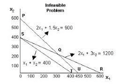
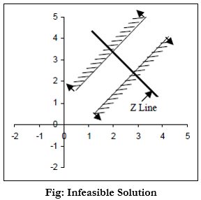
In linear programming, an infeasible solution refers to a solution that does not satisfy all of the constraints of the problem. That is, there is no feasible point in the decision space that satisfies all of the constraints and objective function simultaneously.
An infeasible solution can occur for a variety of reasons, such as when the constraints are contradictory or when the feasible region is empty. When solving a linear programming problem using methods such as the simplex method, an infeasible solution is usually detected during the initialization phase, where artificial variables are introduced to create an initial feasible solution. If no feasible solution can be found, the problem is said to be infeasible.
It is important to identify infeasible solutions early in the problem-solving process to avoid wasting time and resources on an unsolvable problem. Infeasible solutions can also provide insights into the nature of the problem and may help to identify issues with the problem formulation.
When an infeasible solution is identified, the problem may be modified by adjusting the constraints or objective function to make it feasible. Alternatively, the problem may need to be abandoned if it is not possible to find a feasible solution that satisfies the problem requirements.
In summary, an infeasible solution in linear programming refers to a solution that does not satisfy all of the constraints of the problem. It is important to identify infeasible solutions early in the problem-solving process and to modify the problem formulation if necessary to make it feasible.
UNBOUNDED SOLUTION IN SIMPLEX METHOD
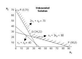
In linear programming, an unbounded solution occurs when the objective function can be increased or decreased indefinitely without violating any of the constraints. In other words, the feasible region is infinite in at least one direction.
An unbounded solution can occur when the feasible region is unbounded, which means that it extends infinitely in one or more directions. This can happen, for example, when there are no upper bounds on some of the decision variables. Alternatively, an unbounded solution can also occur when the objective function is parallel to one of the constraint boundaries.
When solving a linear programming problem using the simplex method, an unbounded solution can be detected during the iteration process by observing that the objective function can be improved indefinitely without violating any of the constraints. In this case, the simplex method cannot find an optimal solution, and the problem is said to be unbounded.
It is important to identify unbounded solutions because they indicate that the problem has no optimal solution. In this case, the decision maker may need to adjust the problem formulation by introducing additional constraints or changing the objective function to make the problem bounded.
In summary, an unbounded solution in linear programming occurs when the feasible region is unbounded or when the objective function is parallel to one of the constraint boundaries. It is important to identify unbounded solutions because they indicate that the problem has no optimal solution, and the problem formulation may need to be adjusted to make it bounded.
OBJECTIVE FUNCTION LINEAR PROGRAMMING
In linear programming, the objective function is a mathematical expression that represents the goal or objective of the problem. It is typically a linear function of the decision variables and is either maximized or minimized subject to the constraints of the problem.
The objective function represents the quantity that the decision maker wants to optimize or minimize, such as profit, cost, or resource utilization. The decision variables represent the inputs or decisions that affect the objective function, such as the amount of resources allocated to different activities or the quantity of goods produced.
The form of the objective function depends on the nature of the problem and the decision maker’s goals. For example, in a profit maximization problem, the objective function might be expressed as the total revenue minus the total cost of production. In a resource allocation problem, the objective function might be expressed as the total utilization of resources subject to constraints on the availability of those resources.
The objective function is an important part of the linear programming problem because it determines the direction in which the decision maker wants to move in the decision space. Maximization problems seek to increase the value of the objective function, while minimization problems seek to decrease it. The constraints of the problem limit the feasible region of the decision space and ensure that the decision variables remain within certain bounds.
In summary, the objective function in linear programming is a mathematical expression that represents the goal or objective of the problem. It is typically a linear function of the decision variables and is either maximized or minimized subject to the constraints of the problem. The form of the objective function depends on the nature of the problem and the decision maker’s goals.
Example: In manufacturing process, the aim may be to maximize the profit or to minimize the loss or cost.
The objective function of each LPP is expressed in terms of decision variables to optimize the criterion of optimality such as cost, profit, revenue, distance etc. i.e. maximize or minimize function.
For instance: In the following problem,
Maximize Z= 15x+10y
Subject to constraints= 2x+3y≤180
x+8y≤60
8x+y≤40
x,y≥0
Objective function is Maximize Z= 15x+10y
CONSTRAINTS IN LPP
Constraints describes the limitations that restrict our choices for decision variables. The constraint may be problem constraints and non-negativity constraints.
Problem constraints: The linear inequalities that are derived from the application. For example: There may be only 40 hours a machine can be used in a week. So the total time, it use would have to be ≤40. The problem constraints are usually stated in a story problem.
Non-negativity constraints: These constraints require that the decision variables be non-negative, i.e., they cannot take negative values. For example, if x represents the number of units of a product to produce, a non-negativity constraint would be x ≥ 0.
Equality constraints: These constraints require that a linear combination of the decision variables be equal to a given constant. For example, if x and y represent the quantities of two different products to produce, an equality constraint could be 2x + 3y = 10.
Inequality constraints: These constraints require that a linear combination of the decision variables be less than or greater than a given constant. For example, if x and y represent the quantities of two different products to produce, an inequality constraint could be 2x + 3y ≤ 10.
Upper and lower bounds: These constraints restrict the range of values that a decision variable can take. For example, if x represents the number of units of a product to produce, an upper bound constraint could be x ≤ 100, indicating that the maximum number of units that can be produced is 100.
Integer constraints: These constraints require that the decision variables take integer values. For example, if x represents the number of units of a product to produce, an integer constraint would be x ∈ Z, indicating that x must be an integer.
Binary constraints: These constraints require that the decision variables take values of 0 or 1. For example, if x represents whether to produce a product or not, a binary constraint would be x ∈ {0,1}, indicating that x can only take the values of 0 or 1.
These are some of the common types of constraints in LPP. The choice of constraint type depends on the specific problem and the nature of the decision variables.
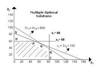
MULTIPLE OPTIMAL SOLUTION IN SIMPLEX METHOD
The optimal solution of any LPP occurs at vertices of feasible area and is unique, in general. In some cases, LPP may have more than one solution yielding the same optimal value of objective function. Each optimal solution is termed as alternative optimal solution.
The alternative optimal solution exists under the following circumstances:
- The objective function is parallel to a constraint that forms the boundary of feasible region.
- The constraint forming the boundary should be active. Equality constraint is always active. The Inequality constraint is active if it passes through extreme points of feasible area.
The number of alternative solutions may be finite or infinite.
DIFFERENCE BETWEEN INFEASIBLE AND UNBOUNDED SOLUTION
| INFEASIBILITY | UNBOUNDEDNESS |
| It is a problem that has no solution. | It is a problem where the constraints do not restrict the objective function and the optimal function or solution goes to infinity. |
| It may stems from an error in specifying some of the constraints in models or from some wrong numbers in data. | This can happen if a problem is being solved with the wrong optimisation sense. |
DEGENERACY IN LPP
Degeneracy in linear programming occurs when the basic variables in the simplex tableau are zero. This means that there is more than one basic variable that could enter the basis, leading to multiple optimal solutions, and potentially slowing down the convergence of the simplex method.
Here are some causes of degeneracy in linear programming:
- Redundant constraints: These are constraints that do not contribute to defining the feasible region. They are either linearly dependent on other constraints or are infeasible. Redundant constraints can lead to degeneracy by reducing the dimensionality of the problem.
- Multiple optimal solutions: When there are multiple optimal solutions, it is possible that some of the basic variables may be zero. This can lead to degeneracy in the simplex method.
- Cycling: Cycling occurs when the simplex method revisits a previous basic feasible solution without making any progress towards the optimal solution. Cycling can occur when there are degenerate basic feasible solutions, making it difficult for the simplex method to move towards the optimal solution.
Here are some methods to overcome degeneracy in linear programming:
- Perturbation: Perturbation involves adding a small amount of noise to the problem to break the degeneracy. This noise can be added to the right-hand side of the constraints or the objective function.
- Bland’s rule: Bland’s rule is a pivot rule used in the simplex method that avoids cycling by selecting the entering variable with the smallest index among the eligible candidates. This guarantees that the pivot variable will always be selected in a deterministic and consistent manner.
- Lexicographic rule: The lexicographic rule is another pivot rule that can be used to avoid cycling by selecting the entering variable based on a predetermined order of priorities.
Overall, degeneracy can cause problems in the simplex method and lead to slower convergence, so it is important to be aware of this phenomenon and take appropriate steps to overcome it.
TWO PHASE SIMPLEX METHOD IN OPERATIONS RESEARCH
The two-phase simplex method is a variation of the simplex method used to solve linear programming problems that involve constraints with inequality signs (i.e., ≤ or ≥). It is used when the problem has a non-feasible basic feasible solution, meaning there is no initial basic feasible solution that satisfies all the constraints.
The two-phase simplex method involves two phases.
First phase: The first phase involves finding a feasible basic feasible solution. To do this, we introduce artificial variables and add them to the constraints with inequality signs. We then solve this modified problem using the simplex method until we reach a basic feasible solution with all artificial variables equal to zero. If the optimal value of the objective function in this phase is greater than zero, then the problem is infeasible.
Second phase: In the second phase, we remove the artificial variables and solve the original problem using the simplex method starting from the basic feasible solution obtained in the first phase. The optimal solution obtained in the second phase is the optimal solution to the original problem.
The two-phase simplex method can be summarized in the following steps:
- Convert the linear programming problem to standard form by introducing slack variables for ≤ constraints and surplus variables for ≥ constraints.
- If there are any constraints with inequality signs, introduce artificial variables to convert them to equality constraints. Add these artificial variables to the objective function with a large coefficient (e.g., M).
- Solve the modified problem using the simplex method to obtain a basic feasible solution. If the optimal value of the objective function is greater than zero, the problem is infeasible.
- Remove the artificial variables from the problem and solve the original problem using the simplex method starting from the basic feasible solution obtained in step 3.
- If the optimal value of the objective function in step 4 is finite, it is the optimal value of the original problem. If it is infinite, the original problem is unbounded.
The two-phase simplex method can be computationally expensive, especially for large problems. However, it guarantees that a feasible solution will be found if one exists.
REPLACEMENT RATIO IN LINEAR PROGRAMMING
The replacement ratio is a concept in linear programming that is used in the context of decision-making for replacing or upgrading assets or resources. It is a measure of the relative efficiency or profitability of replacing an old asset with a new one, or upgrading an existing asset.
The replacement ratio is calculated by dividing the increase in revenue resulting from the replacement or upgrade by the cost of the replacement or upgrade. More formally, the replacement ratio can be expressed as:
Replacement Ratio = (Increase in Revenue) / (Cost of Replacement or Upgrade)
In a linear programming problem, the replacement ratio can be used as a decision variable that is subject to constraints. For example, suppose a company is considering upgrading its manufacturing equipment to improve production efficiency. The decision variable could be the replacement ratio, and constraints could be imposed on the availability of funds for the upgrade and the maximum downtime allowed during the upgrade process.
The objective function in this case would typically be to maximize the increase in revenue resulting from the upgrade while minimizing the cost of the replacement or upgrade. The optimal value of the replacement ratio obtained from solving the linear programming problem would indicate the most efficient or profitable level of replacement or upgrade.
In summary, the replacement ratio is a concept in linear programming that can be used to quantify the efficiency or profitability of replacing or upgrading assets or resources. It can be used as a decision variable in a linear programming problem to optimize the replacement or upgrade process.